While many relationships in our world can be described using a single mathematical function or relation, there are also many that require either more or less than what one equation describes. The behavior being described might start at a specific time, or its nature changes at one or more points in time. Two examples of such situations could be:
 Acceleration up to a speed limit |  Free fall then controlled descent |
In the graph on the left, note that the blue line starts at the origin. It does not appear to the left of the origin at all. Furthermore, when x = 3 the blue line stops and the green line begins – but with a different slope.
In the graph on the right, note that the blue curve starts at x = 0. It does not appear of the left of the vertical axis at all. And when x = 3 the blue parabola turns into a green line with a very different slope. And the green line stops at x = 5.5, just as it reaches the horizontal axis.
These graphs do not seem to follow all the rules you were taught for graphing lines or parabolas. Instead of being defined over all Real values of x, they start and stop at specific values. The graphs also show (in this case) two very different functions, but in a way that makes them look as though they are meant to represent a single, more complex function. Both of these graphs are examples of “Piecewise Functions”, functions defined in a way that lets you mix and match as many separate components (pieces) as you wish.
Steady Rise In Speed Up To a Speed Limit
If a car gradually speeds up from zero to 30 miles per hour, then stays at that speed, the graph of this situation would look like this if each unit on the vertical axis represents 10 miles per hour, and the horizontal axis represents time:
This can be modeled mathematically using a piecewise function:

Interpreting The Notation
Note that the definition begins exactly the way all function definitions do, with the name of the function (“f” in this case), followed by a set a parentheses that contains the list of inputs that the function requires (“x” in this case), and an equal sign. Then the fun starts…
To the right of the equal sign is a large curly brace, which serves as a vertical grouping symbol to contain the component parts of the piecewise function definition.
To the right of the curly brace are all the “pieces” of the function, as many as may be needed. In this case, two pieces are needed. Each line to the right of the curly brace contains two things: a function definition, and a “domain restriction”. The function definition part is hopefully something you are thoroughly familiar with by now. The domain restriction indicates which values of “x” this definition applies to.
In the example above, the first piece only applies to “x” values that are greater than zero and less than three. If the value of “x” lies within that range , then we should use the definition

to produce the result of the function. If the value of “x” is greater than or equal to three, then we should use the definition

If the value of “x” is zero or less, this function will not produce a result, so the graph will not show any points to the left of the origin.
If you examine the graph above, you will see that this is exactly what is graphed: a line with a slope of 1 and a y-intercept of zero for x values between zero and three (the blue line), then a horizontal line with a slope of zero at y=3 for all x values of three or greater (the green line). The blue line is a graphical representation of the first line of the piecewise definition, while the green line represents the second line of the piecewise definition.
Free Fall Followed By A Controlled Descent
Suppose an object falls freely through the air towards the earth for three seconds, at which time a parachute opens and instantly slows its rate of descent to a constant speed until it hits the ground. This situation could be described by a graph showing the object’s height above the ground on the vertical axis, and elapsed time on the horizontal axis:
This graph can be described using the following piecewise definition:

The first line of the definition describes a parabola that opens down with a vertex at (0,7). But it only applies to “x” values that are greater than zero and less than three. This is represented by the blue curve in the right-hand graph.
The second line of the piecewise definition describes a line with a slope of -1 and a y-intercept of 5.5. But this line does not start until x=3, and it ends at x=5.5. This is represented by the green line on the right-hand graph.
This graph illustrates how two very different types of functions can be combined to form a single piecewise function. A piecewise function is able to describe a complex and varying behavior perfectly, something that a single function is not able to do when the mathematical nature of the behavior changes over time.
There Are Few Constraints
Piecewise definitions can include any kind of mathematical relations or functions you wish to include: polynomial, trigonometric, rational, exponential, etc.
The individual pieces of the definition do not have to connect to one another if you do not wish them to… there can be huge gaps (vertical, horizontal, or both) in the graph between where one piece ends and the next begins, or no gaps if every piece connects smoothly to the next. It can be a fun challenge to figure out the equation needed to ensure that one piece connects smoothly to the next.
The one constraint that may apply is based on the vocabulary being used. If the word that follows “piecewise” is “function”, then the complete piecewise definition must not produce more than one result for any input value of “x”. It should produce either no result or one result for all possible input values. If a piecewise definition produces more than one result for any value of “x”, it must be called a “piecewise relation”, not a “piecewise function”.
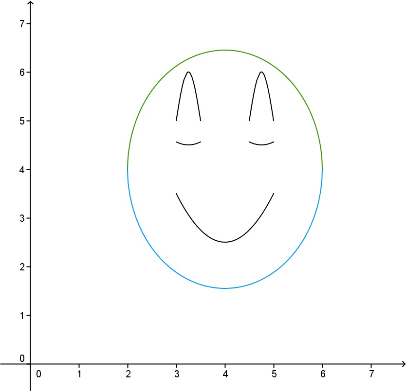
Piecewise definitions can be used to have some fun too, as has been done with this piecewise relation. Scroll to the bottom of this page to see its graph:


