Using Corresponding Points to Determine Dilation Factors and Translation Amounts

Two earlier posts provide background information for this one: Function Translations and Function Dilations. If you are not already familiar with these topics, you may benefit from reading those first.

Given two points on a curve and their corresponding points after transformation, how does one determine the underlying transformations? Since two dilations and two translations may be taking place, it can be complex to try to separate the effects of dilation from those of translation.

As an example, consider the two curves above. The green curve is the graph of

$y_1(x_1)~=~(x_1 -1)^2+1$

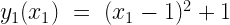
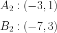
and the red curve is a transformation of the green one. Two points are labeled on the green curve:

$A_1:(1,1)\\*~\\* B_1:(2,2)$

and their corresponding transformed points are labeled on the red curve:

$A_2:(-3,1)\\*~\\* B_2:(-7,3)$

The challenge is to determine what combination of horizontal and vertical transformations turn the green graph into the red one, and from there determine the equation of the transformed graph.

Finding the Horizontal Transformation

Dilations result from multiplication (or division), and translations result from addition (or subtraction). Combining the two transformations produces the equation:

$dx_1+t~=~x_2$

Or, verbally, the original x-coordinate $x_1$ has been dilated by a factor d, then translated by t, to produce the transformed x-coordinate $x_2$ . The order of operations forces us to apply the dilation factor before adding the translation amount.

We can now use the pair of points on the green curve and their corresponding transformed points on the red curve to solve for d and t. Looking only at the x-coordinates of the points and their transformations, we see that

1 => -3
2 => -7

and we can substitute each of these pairs into the equation above to produce a system of two equations and two unknowns:

$\begin{cases}d(1)+t~=~-3\\*d(2)+t~=~-7\end{cases}$

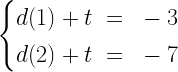
Solving this system by subtracting the two equations produces:

$-d~=~4\\*~\\*~~d~=~-4$

and substituting this result back into the first equation produces:

$(-4)(1)+t~=~-3\\*~\\*~~~~~~~~~~~~~~~t~=~1$

so the horizontal transformation of the green function that produces the red function is:

$~~~~dx_1+t~=~x_2\\*~\\*-4x_1+1~=~x_2$

Finding the Vertical Transformation

Using the same reasoning about the nature of dilations and translations, and the same approach as above, the vertical transformation can be modeled using the equation:

$dy_1+t~=~y_2$

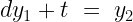
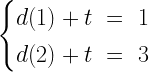
and the two sets of y-coordinates from the green points and their corresponding transformed red points:

1 => 1
2 => 3

which lead to the two equations:

$\begin{cases}d(1)+t~=~1\\*d(2)+t~=~3\end{cases}$

and their solution:

$-d~=~-2\\*~\\*~~~d~=~2$

$(2)(1)+t~=~1\\*~\\*~~~~~~~2+t~=~1\\*~\\*~~~~~~~~~~~~t~=~-1$

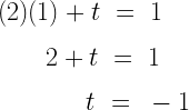
so the vertical transformation of the green function that produces the red function is:

$~dy_1+t~=~y_2\\*~\\*2y_1-1~=~y_2$

The Transformed Function

Now that we have calculated the two transformations

$-4x_1+1~=~x_2\\*~\\*~~~2y_1-1~=~y_2$

what is the equation of transformed red graph? The green graph has the equation:

$y_1~=~\mathbf{(x_1 -1)^2+1}$

so we can apply the vertical transformation to it by substituting the equation above into the transformation equation for $y_1$ above:

$2\{\mathbf{(x_1 -1)^2+1}\}-1~=~y_2$

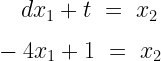
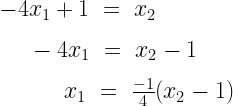
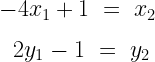
then apply the horizontal transformation… but there is one more step needed before we can do so. Note that the equation for the green graph above has an $x_1$ in it, but our horizontal transformation equation above is solved for $x_2$ . So, we need to solve it for $x_1$ ,

$-4x_1+1~=~x_2\\*~\\*~~~~~-4x_1~=~x_2-1\\*~\\*~~~~~~~~~~x_1~=~\frac{-1}{4}(x_2-1)$

The steps above convert the transformation equation from a form where the dilation factor (-4) and translation amount (+1) are both easily read directly

$-4x_1+1~=~x_2$

into the form you are used to seeing for horizontal transformations, where the reciprocal of the horizontal dilation factor and the negative of the horizontal translation amount appear

$x_1~=~\mathbf{\frac{-1}{4}(x_2-1)}$

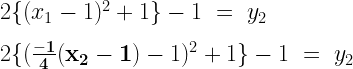
We can now subsitute the above for $x_1$ in the equation that resulted from applying the vertical transformations. The substituted text is in bold:

$2\{(x_1 -1)^2+1\}-1~=~y_2\\*~\\*2\{(\mathbf{\frac{-1}{4}(x_2-1)} -1)^2+1\}-1~=~y_2$

And we have finally arrived at the equation for the red graph $y_2(x_2)$ , expressed as vertical and horizontal transformations of the green graph $y_1(x_1)$ :